6 Part III: Creating and Joining Datasets
Moose density and browsing preferences
The team of researchers were curious if moose browsing preferences changed depending on moose density. They hypothesized that at
At low moose densities: browsing would be selective, with moose favoring the most palatable tree species.
At high moose densities: Would have high competition, and browsing pressure would become less selective, with moose consuming all sapling species more uniformly.
In this section, we will merge the Moosedataand the Sapling datasets, to explore how browsing intensity on different tree species correlates with moose density across ecoregions. You will practice using the left_join() function to combine these dataset
Question 21
a) Using the original moose_clean dataset, filter() function to select only the rows for the year 2020. Then create a new column called MooseDensity using the mutate() function. Save the dataset under a new name called moose_2020b. (HINT: you previously did this for question 9)
- Use
left_join()to joinmoose_2020bwith thesap_cleandataset, matching rows by the commonEcoregioncolumn. Save the result asmoose_sap.
Question 22
Using the dataset you just created, calculate the average browsing score and average moose density for each species within each ecoregion.
With the help of pipes %>% , group_by Species and Ecoregion, then use summarize() to find the mean() BrowsingScore, and then find the mean() MooseDensity. Print the result using the print() function. Save the result as sum_spe_browse. HINT: There is example code using pipes %>% in Questions 12 and 18 above.
Question 23
The research team created the following figure to help visualize how average browsing intensity on different tree species changes with moose density across ecoregions. The graph uses the ggplot2 package, which is beyond the scope of this assignment. However, if you would like, you can copy and paste the code below into your R console to explore the plot.
library(ggplot2)

ggplot(sum_spe_browse, aes(x = AvgDensity, y = AvgBrowsing, color= Species)) +
  geom_point(size = 3) +

  theme_minimal() +
  labs(title = "Browsing Intensity Across Moose Density by Species",
       x = "Average Moose Density",
       y = "Average Browsing Score")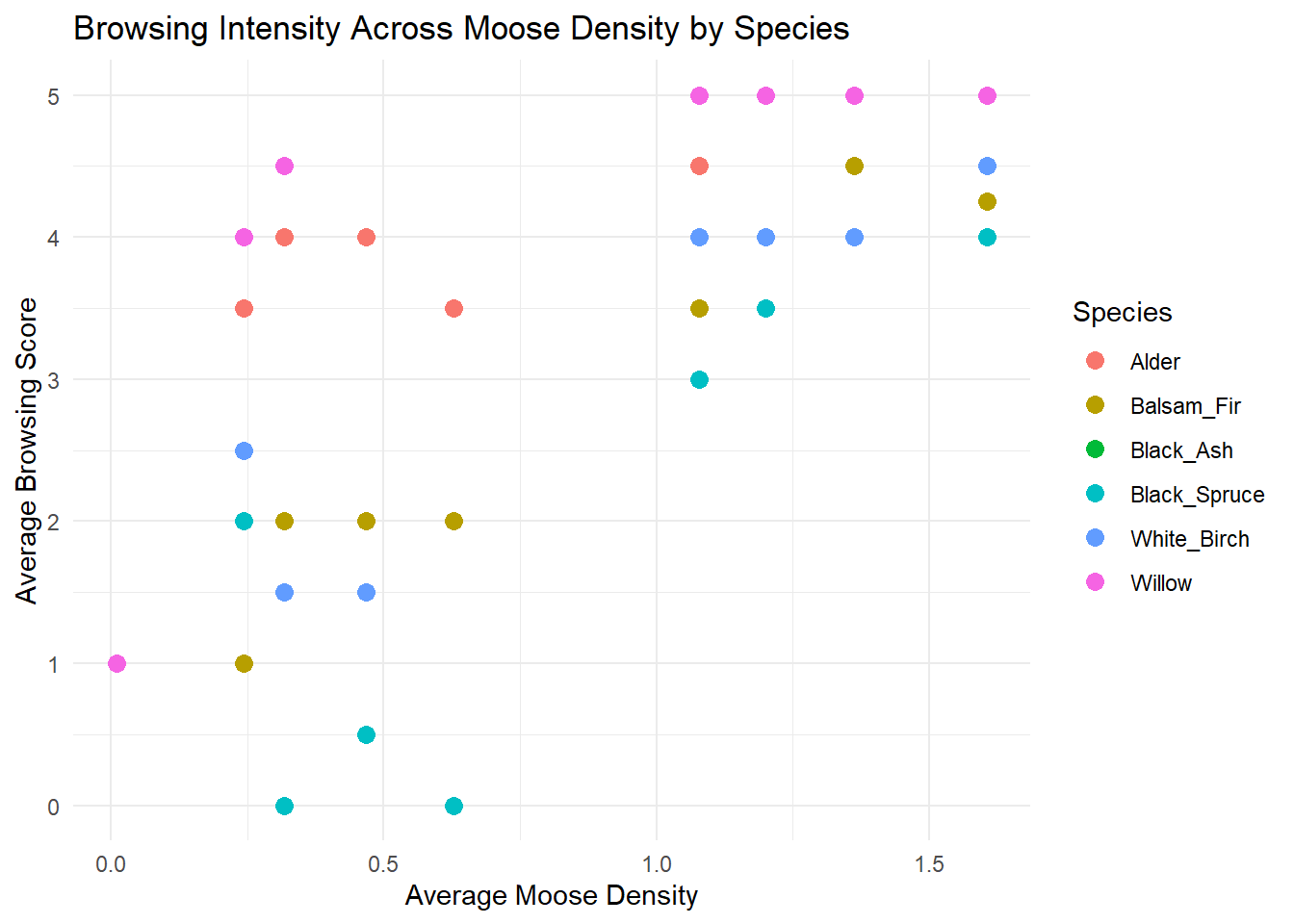
Based on the figure, answer the following questions using 1-2 sentences.
- Is there evidence that supports the researchers’ hypothesis? Do moose show strong preferences at low density and shift to more generalist browsing at higher density? Add a short comment (1-2 sentences) with your answer.
- Which sapling specie(s) do moose favour the most? Which do they browse the least? Add a short comment (1-2 sentences) with your answer.
- Which sapling species is not shown on the figure and why? Add a short comment (1-2 sentences) with your answer.
6.0.1 Moose-vehicle collisions
As moose populations expanded across Newfoundland in the 20th century, so did the frequency of moose-vehicle collisions. These incidents pose serious risks to both humans and wildlife, especially in regions where roads intersect key moose habitat.
In this section, you’ll explore a simplified dataset containing the number of recorded moose-vehicle collisions per ecoregion in 2020. Your goal is to investigate whether moose density in an ecoregion can help explain collision patterns.
Question 24
Copy and paste each vector below, then run them so they appear under your Values section in the Envionment.
Then add a line of code (example given below) where you use the data.frame() function to create a dataset using your vectors. Save this dataset as moose_coll.
collisions2020 <- c(56, 60, 14, 36, 48, 10, 40, 110, 6)
human_pop <- c(18000, 12000, 4000, 75100, 24000,3500, 32000, 270000,    2300)
study_sites <- c("North_Shore_Forests","Northern_Peninsula_Forests", "Long_Range_Barrens","Central_Forests","Western_Forests","EasternHyperOceanicBarrens","Maritime_Barrens","Avalon_Forests","StraitOfBelleIsleBarrens")

moose_coll <- data.frame(collisions2020, human_pop, study_sites)
Question 25
Now we would like to join this dataset with moose_2020 (from Part One, question 9). This would allow us to investigate how moose density plays into collisions across our study sites. However, if we try to use left_join() to join them, we will encounter an error. This is because the name of the regions in the moose_2020 dataset is under Ecoregion while our moose_coll dataset stores them under study_sites.
To correct this and join our datasets we can use the
rename_with()function. Here is some template code that you can adapt to make the necessary change. Rename the column holding site information in themoose_colldataset and save the renamed result asmoose_coll2.Template: rename_with(NewName = OldName)
Now join the datasets into a new dataset using
left_join(). Save the joined dataset ascoll_merge. HINT: follow the template of the code you used above in question 21.
Question 26
a. How does moose density relate to the number of moose-vehicle collisions? Use the plot() function to create a scatterplot of MooseDensity and collisions2020
- What trends do you see? Are there any outliers? Write 1-2 sentences as a comment.
Question 27
Which ecoregions have the highest number of moose collisions per person? Create a new column called coll_per_capita that is equal to collisions2020 divided by human_pop. HINT: Use the mutate function as you did in Part I, question 6, but with appropriate variables. Save the dataset with the new coll_per_capita column as coll_merge_per_capita.
Question 28
Use the plot() function to create a scatterplot of coll_per_capita versus human_pop
Question 29
Write 1-2 sentences describing what trends you see. Does this trend make sense based on what you know about moose and human populations in Newfoundland?